Markov Chains: A Practitioner's Refresher

Markov Chains appear throughout quantitative finance: regime-switching models for asset returns, credit rating migration matrices, Hidden Markov Models for signal detection, and any system where the probability of transitioning to the next state depends only on the current state. This post walks through the core mechanics — transition matrices, multi-step probabilities, forecasting, and stationary distributions.

Definition

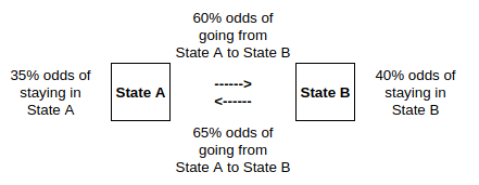
A Markov Chain is a stochastic process describing a sequence of possible events in which the probability of each event depends only on the state attained in the previous event.

Formally:

• Let $s_t$ be a random variable taking values in $\{1, 2, \ldots, N\}$
• Let $a_{i,j} = \mathbb{P}(s_t = j \mid s_{t-1} = i)$ denote the transition probability from state $i$ to state $j$
• $s_t$ is a Markov Chain if $\mathbb{P}(s_t = j \mid s_{t-1} = i, s_{t-2} = k, \ldots) = \mathbb{P}(s_t = j \mid s_{t-1} = i) = a_{i,j}$

The state dynamics are fully specified by the transition matrix:

$$A = \begin{bmatrix} a_{1,1} & \cdots & a_{1,N} \\ a_{i,1} & \cdots & a_{i,N} \\ a_{N,1} & \cdots & a_{N,N} \end{bmatrix}$$

Since the elements of each row must sum to unity:

$a_{i,1} + \cdots + a_{i,N} = 1$

State Vectors

Let $e_i$ denote the $i$-th row vector of the $N \times N$ identity matrix. Let $\xi_t$ denote a $1 \times N$ row vector that equals $e_i$ when the state $s_t$ is equal to $i$:

$\xi_t = (0, \ldots, 0, \underbrace{1}_{i\text{-th element}}, 0, \ldots, 0)$

The expectation of $\xi_{t+1}$ is a vector whose $j$-th element is the probability that $s_{t+1} = j$:

$\mathbb{E}(\xi_{t+1} \mid s_t = i) = (a_{i,1}, \ldots, a_{i,N})$

We infer that $\mathbb{E}(\xi_{t+1} \mid s_t = i) = \xi_t \mathbf{A}$, or more generally $\mathbb{E}(\xi_{t+1} \mid \xi_t) = \xi_t \mathbf{A}$, and since $s_t$ follows a Markov Chain:

$\mathbb{E}(\xi_{t+1} \mid \xi_1, \ldots, \xi_t) = \xi_t \mathbf{A}$

In plain English: when $s_t = i$, $\xi_t$ selects the $i$-th row of the identity matrix. Multiplying by the transition matrix $\mathbf{A}$ extracts the corresponding row of transition probabilities. Because the chain is Markov, only the current state matters — all the history is irrelevant. It’s really just a structured way to look up the right transition probabilities.

Two-Step Transition Probabilities

The probability that $s_{t+2} = j$ given $s_t = i$ is:

$\mathbb{P}(s_{t+2} = j \mid s_t = i) = a_{i,1}a_{1,j} + \cdots + a_{i,N}a_{N,j}$

This is the $(i, j)$ element of $\mathbf{A}^2$. Intuitively, to get from state $i$ to state $j$ in two steps, we sum over all possible intermediate states — weighting each path by the product of its transition probabilities.

N-Step Transition Probabilities

In general, the probability that $s_{t+m} = j$ given $s_t = i$ is the $(i, j)$ element of $\mathbf{A}^m$:

$\mathbb{E}(\xi_{t+m} \mid \xi_t, \xi_{t-1}, \ldots, \xi_1) = \xi_t \mathbf{A}^m$

We locate the appropriate entry in the transition matrix raised to the $m$-th power.

Forecasting Transitions

Assume we have received information $I_t$ up to date $t$. Let

$\pi_t = [\mathbb{P}(s_t = 1 \mid I_t), \ldots, \mathbb{P}(s_t = N \mid I_t)]$

denote the conditional probability distribution over the state space. Since $\pi_t = \mathbb{E}(\xi_t \mid I_t)$, we infer that

$\pi_{t+1} = \mathbb{E}(\xi_{t+1} \mid I_t) = \mathbb{E}(\xi_t \mid I_t) \mathbf{A}$

If $I_t$ contains no leading information, the forecast state distribution is:

$\pi_{t+1} = \pi_t \mathbf{A}$

The one-step-ahead conditional distribution is the current distribution multiplied by the transition matrix. All the information is already embedded in $\pi_t$.

Stationary Distributions

A distribution $\pi$ is stationary if it satisfies $\pi = \pi \mathbf{A}$ — the forecast distribution is the same as the current one. If the Markov Chain is ergodic, the system

$$\begin{aligned} \pi &= \pi \mathbf{A} \\ \pi \iota &= 1 \end{aligned}$$

has a unique solution, where $\iota$ denotes the $N \times 1$ vector of ones. This stationary distribution is the long-run proportion of time spent in each state, regardless of the starting point — a property that makes it central to equilibrium analysis in credit models, economic regime models, and any setting where we care about steady-state behaviour.

Where This Shows Up in Practice

The machinery above is the scaffolding behind several standard tools in quantitative finance:

• Regime-switching models for asset returns (Hamilton, 1989) treat the economy as a Markov chain over latent states — typically a “high-volatility” and “low-volatility” state — and use maximum likelihood or Bayesian inference to back out the transition probabilities from observed returns.
• Credit rating migration matrices published by rating agencies are transition matrices for a Markov chain over rating categories. The n-step probability calculation gives the distribution of likely ratings n years from today, which feeds directly into credit portfolio risk models.
• Hidden Markov Models extend the framework by treating the state as unobservable and the observed data (returns, volumes) as emissions from the hidden state. HMMs are used for trade classification, market microstructure analysis, and anomaly detection.

In all three applications, the stationary distribution tells you the long-run proportion of time the system spends in each state — a quantity that matters for setting capital reserves, computing unconditional risk premia, and understanding the base-rate behaviour of the system you’re modelling.