Measuring Factor Exposure
How to use factor regressions to measure a stock's or portfolio's exposure to systematic risk premia — and why a hedge fund manager and an ETF provider care about the same regression for opposite reasons.
In the first post in this series, we introduced risk factors in finance and explored their history. In the second post, we examined the traditional factor exposures — Size, Value, Momentum, Profitability, Investment — individually, charting their return patterns. This article shifts focus to measuring how much of a stock’s or portfolio’s return is explained by these factors, and why that measurement matters.
Why Factor Exposure Might Matter to You
Consider two scenarios.
Scenario 1: The hedge fund manager. You employ traders or portfolio managers with superior stock-picking skill, and you expect their returns to have low or no correlation with the market. You might go further: “Not only do I want returns uncorrelated with the market, I want them uncorrelated with well-known risk premia like Momentum.” Factors are risk premia — they hypothesise that bearing a certain risk earns a certain compensation. You’re not paying your PMs to harvest risk premia that anyone can access through a cheap ETF. You want returns that are not explainable by a factor model, and this unexplainable return is often called “alpha.”
Scenario 2: The ETF provider. You issue and oversee a range of funds designed to replicate returns closely aligned with Value, Size, Momentum. A client raises concerns that your “US Value ETF” doesn’t have sufficiently significant beta to the Value factor’s hypothetical returns. This could be due to a poorly specified investment approach, or style drift. You need — both qualitatively and quantitatively — to validate that your fund is replicating Value returns as intended.
In both scenarios, factor regressions are the tool.
What Are We Measuring?
Let’s revisit the Fama-French Three Factor model:
where:
- is the return of asset at time
- is the risk-free rate at time
- is the sensitivity of asset to the market factor
- is the return on the market portfolio at time
- is the return difference between small and large firms at time
- is the sensitivity of asset to the SMB factor
- is the return difference between high and low book-to-market equity firms at time
- is the sensitivity of asset to the HML factor
- is the idiosyncratic error term
This model asserts that all returns () are composed of some amount () of market return, some amount () of Size return, some amount () of Value return, plus random variation () that averages to zero. But that contradicts what our hedge fund manager wants. We can add an alpha term:
The Three Factor model always implicitly had this term — it just claimed , so it wasn’t shown.
The hedge fund manager wants to measure alpha and verify it isn’t zero. If their trader’s alpha turns out to be zero — or not significantly different from zero — all their returns are explained by the Three Factor model and they should be fired.
The ETF provider wants to measure the factor beta and verify it is significant. It’s not enough for their fund to have some Value exposure — they need to show the exposure coefficient is statistically significant.
We’ll use Ordinary Least Squares (OLS) regressions to measure these values. There are more rigorous specification tests one could run, but OLS with HAC standard errors is a reasonable starting point.
Factor Regressions
To perform a factor regression, we need factor return data and stock or portfolio data. Here’s the boilerplate Python code:
# Returns monthly log returns (computed from end-of-month prices)
def get_stock_log_returns(ticker):
    data = yf.download(ticker, interval='1d', progress=False)['Close']
    data = data.resample('1m').last().iloc[:-1]
    log_returns = np.log(data.pct_change() + 1).dropna()
    log_returns.name = ticker
    return log_returns

def get_ff_data(data, start='1-1-1960'):
    factor_data = pdr.get_data_famafrench(data, start)[0]
    factor_data.index = (factor_data.index.to_timestamp() + MonthEnd(0)).date
    factor_data.index = pd.to_datetime(factor_data.index)
    return factor_data

def merge_stock_and_ff_data(stock_log_rets, factor_data):
    return pd.concat([stock_log_rets * 100, factor_data], axis=1).dropna()

def gather_stock_factor_data(ticker='AAPL', factor_data='F-F_Research_Data_5_Factors_2x3'):
    stock_data = get_stock_log_returns(ticker)
    ff_data = get_ff_data(factor_data)
    merged_data = merge_stock_and_ff_data(stock_data, ff_data)
    return merged_data
Running gather_stock_factor_data('AMZN') produces:
| AMZN | Mkt-RF | SMB | HML | RMW | CMA | RF | |
|---|---|---|---|---|---|---|---|
| 2023-02-28 | -9.03 | -2.58 | 0.69 | -0.78 | 0.9 | -1.4 | 0.34 |
| 2023-03-31 | 9.18 | 2.51 | -7.01 | -9.01 | 1.92 | -2.29 | 0.36 |
| 2023-04-30 | 2.07 | 0.61 | -2.56 | -0.03 | 2.31 | 2.85 | 0.35 |
| 2023-05-31 | 13.41 | 0.35 | -0.43 | -7.8 | -1.76 | -7.2 | 0.36 |
| 2023-06-30 | 7.8 | 6.46 | 1.33 | -0.2 | 2.2 | -1.75 | 0.4 |
Now we need the OLS regression:
def point_in_time_regression(ticker, start_date='1960-01',
                              end_date=datetime.datetime.now().date()):
    merged_data = gather_stock_factor_data(ticker)
    merged_data = merged_data.loc[start_date:end_date]
    endog = merged_data[ticker] - merged_data.RF.values
    exog_vars = [item for item in list(merged_data.columns)
                 if item not in [ticker, 'RF']]
    exog = sm.add_constant(merged_data[exog_vars])

    ff_model = sm.OLS(endog, exog).fit()
    ff_model = ff_model.get_robustcov_results(cov_type='HAC', maxlags=1)

    print(ff_model.summary())

    fig = sm.graphics.plot_partregress_grid(
        ff_model, fig=plt.figure(figsize=(12, 8)))
    plt.show()
Testing on AAPL using the Three Factor model from 2005 onwards:
point_in_time_regression(
    ticker='AAPL',
    factor_data='F-F_Research_Data_Factors',
    start_date='2005'
)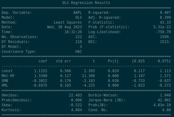
There are a lot of figures here, but the key panel is:
The rows are the explanatory variables. “const” is the alpha term. The columns:
- coef: the beta coefficient — the proportion of how much each explanatory variable contributes to the return
- std err: standard error — one standard deviation of variation around the coefficient
- t: the test statistic
- P > |t|: the p-value
- [0.025 — 0.975]: the 95% confidence interval
Plugging these values in:
The regression estimates that:
- AAPL shows positive alpha of 1.1152, statistically significant at the 5% level
- AAPL’s market beta is approximately 1.339 — it moves more than the market
- AAPL has a negative, significant relationship to the Size factor. This makes sense: the Size factor rewards owning small companies, and Apple is enormous
- AAPL has a negative, significant relationship to the Value factor. Again sensible: the Value factor rewards companies with high book-to-market ratios, and Apple’s book-to-market ratio is tiny
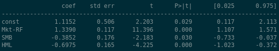
This was probably expected. Berkshire Hathaway should look different:
- BRK-A shows positive alpha of 0.2059, but it’s not statistically significant — we cannot reject the null hypothesis that the true alpha is zero (p = 0.419)
- BRK-A’s market beta is 0.72, so it moves less than the market
- BRK-A has strong negative exposure (-0.46) to Size — like Apple, Berkshire is huge
- BRK-A has strong positive exposure (0.34) to Value, consistent with its reputation as a value-oriented holding company
Back to the Scenario
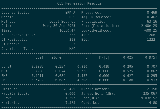
At the beginning of the article we outlined a scenario where our “US Value ETF” was drawing concerns. The S&P 500 provides a baseline:
The S&P 500 has a 0.0181 beta coefficient to Value, which is marginally significant (p = 0.06) — at conventional thresholds we’d fail to reject the null of zero exposure. Now compare with iShares MSCI USA Value ETF (VLUE):
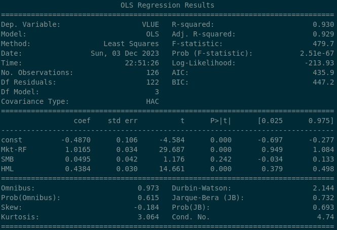
The Value factor exposure is dramatically different: a beta coefficient of 0.4384, strongly statistically significant. Over the long run, this ETF clearly exposes its owners to the Value factor. The partial regression plot confirms it:
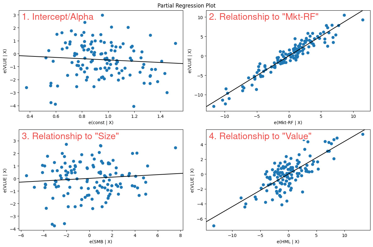
In the bottom-right panel, the line slopes upward from left to right with meaningful steepness — exactly what we want to see for a significant positive factor exposure.
Time-Series Factor Regressions
We may also want to see how this exposure varies through time. The 25th percentile exposure during the period was 0.379 and the 75th percentile was 0.498 — but I always prefer seeing these things visually:
def rolling_regression(ticker, window=60,
                        factor_data='F-F_Research_Data_5_Factors_2x3',
                        start_date='1960-01',
                        end_date=datetime.datetime.now().date()):
    merged_data = gather_stock_factor_data(ticker, factor_data=factor_data)
    merged_data = merged_data.loc[start_date:end_date]
    endog = merged_data[ticker] - merged_data.RF.values
    exog_vars = [item for item in list(merged_data.columns)
                 if item not in [ticker, 'RF']]
    exog = sm.add_constant(merged_data[exog_vars])
    rols = RollingOLS(endog, exog, window=window)
    rres = rols.fit()

    print('Most recent (ending) Beta Coefficients\n\n', rres.params.iloc[-1])
    fig = rres.plot_recursive_coefficient(variables=exog_vars, figsize=(10, 18))
Running on VLUE:
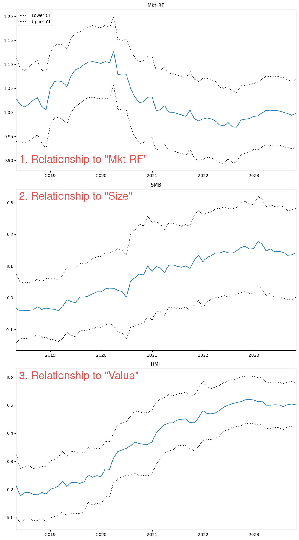
The 5-year rolling beta to Value increased from approximately 0.2 in 2018 to 0.5 in 2023. A longer lookback might provide context, but for now we can see the time-varying nature of factor exposure clearly.
Conclusion
Factor regressions let us validate — or reject — the idea that a fund or investment strategy has exposure to systematic risk factors. In some cases we want that exposure to be large and significant (the ETF provider). In others, we want it to be small and insignificant, implying that our investment outcomes are distinct from known risk premia (the hedge fund manager). Same tool, different objectives.
The code for this post is available on request.