Exploring Traditional Factor Portfolios
Walking through Size, Value, Momentum, Profitability, and Investment factor returns using data from Ken French's library — with code, charts, and observations on crisis-period behaviour.
In the first post in this series, I laid out the theoretical foundation for factor investing. Here I put it to work: pulling data from Ken French’s library, computing cumulative returns, and seeing how each of the traditional factors — Size, Value, Momentum, Profitability, Investment — has actually performed. Some of the results are as expected. Others are more interesting, particularly the crisis-period behaviour of the newer factors.
Getting Data
One of the main sources of data for the traditional risk factors is Ken French’s Data Library. Ken — co-creator of the Fama-French Three Factor Model alongside Eugene Fama — provides a great service to the finance world by curating and offering these data for general use. His data library is used regularly by academics and practitioners alike.
To make gathering these data more convenient, we’ll access them via the getFamaFrenchFactors Python module:
pip install getFamaFrenchFactorsimport getFamaFrenchFactors as gff
# Get the Fama-French three factor model (monthly data)
df_ff3_monthly = gff.famaFrench3Factor(frequency='m')
# Get the Fama-French three factor model (annual data)
df_ff3_annual = gff.famaFrench3Factor(frequency='a')This module provides a convenient wrapper around Ken’s website. If you want to calculate the factor returns yourself and have a WRDS account, the famafrench module can do that. For this post we’ll take the pre-prepared data.
Fama-French Three Factor Model
To recap, the Three Factor model explains stock returns using three1 primary risk factors: market return, the “size” (SMB) factor, and the “value” (HML) factor:
where:
- is the return of asset at time
- is the risk-free rate at time
- is the sensitivity of asset to the market factor
- is the return on the market portfolio at time
- is the return difference between small and large firms at time
- is the sensitivity of asset to the SMB factor
- is the return difference between high and low book-to-market equity firms at time
- is the sensitivity of asset to the HML factor
- is the idiosyncratic error term
We can get all the data with:
import getFamaFrenchFactors as gff
df_ff3_monthly = gff.famaFrench3Factor(frequency='m')
df_ff3_monthly.set_index('date_ff_factors', inplace=True)
The most recent 10 rows (df_ff3_monthly.tail(10)) look like this:
| date_ff_factors | Mkt-RF | SMB | HML | RF |
|---|---|---|---|---|
| 2022-09-30 | -0.0935 | -0.0079 | 0.0006 | 0.0019 |
| 2022-10-31 | 0.0783 | 0.0009 | 0.0805 | 0.0023 |
| 2022-11-30 | 0.046 | -0.034 | 0.0138 | 0.0029 |
| 2022-12-31 | -0.0641 | -0.0068 | 0.0132 | 0.0033 |
| 2023-01-31 | 0.0665 | 0.0502 | -0.0405 | 0.0035 |
| 2023-02-28 | -0.0258 | 0.0121 | -0.0078 | 0.0034 |
| 2023-03-31 | 0.0251 | -0.0559 | -0.0901 | 0.0036 |
| 2023-04-30 | 0.0061 | -0.0334 | -0.0003 | 0.0035 |
| 2023-05-31 | 0.0035 | 0.0153 | -0.078 | 0.0036 |
| 2023-06-30 | 0.0646 | 0.0155 | -0.002 | 0.004 |
The columns represent:
- Mkt-RF: Market return minus risk-free return (the market risk premium). This is the compensation for exposing capital to risk through market investment, versus the alternative of a “safe” asset like a short-term bond2
- SMB: Small Minus Big — the difference in returns between small and large companies
- HML: High Minus Low — the difference in returns between companies with high and low book-to-market ratios
- RF: Risk-free rate
Size (SMB)
Conceptual basis: Small companies tend to yield higher returns compared to large companies. A strategy of buying small companies while selling large companies short should yield favourable returns — hence “small minus big.”
Potential explanatory theories include reduced liquidity in small caps (rewarding liquidity risk), greater growth potential, and more agility requiring less capital to fund a strategic pivot.
def show_me_factor_info(factor, df):
    df_single_factor = df[factor]
    df_single_factor.cumsum().plot(title='{} Factor Cumulative Returns'.format(factor))
    annual_volatility = df_single_factor.std() * (12**0.5)
    mean_annualized_return = df_single_factor.mean() * 12
    print(f"Cumulative Return: {round(df_single_factor.sum()*100, 2)}%"
          f"\nMean Annual Return: {round(mean_annualized_return*100, 2)}%"
          f"\nAnnualised Volatility: {round(annual_volatility*100, 2)}%"
          f"\nAnnual Sharpe Ratio: {round(mean_annualized_return/annual_volatility, 2)}")

show_me_factor_info('SMB', df_ff3_monthly)
Cumulative Return: 219.53%
Mean Annual Return: 2.26%
Annualised Volatility: 10.98%
Annual Sharpe Ratio: 0.21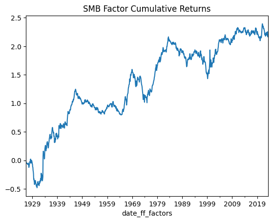
Value (HML)
Conceptual basis: Inexpensively valued companies tend to generate higher returns than their pricier counterparts.
Potential explanatory theories include companies with substantial debt or erratic earnings being undervalued, investor aversion to past underperformers, and the tendency of such companies to revert toward or surpass a 1:1 price-to-book ratio.
show_me_factor_info('HML', df_ff3_monthly)Cumulative Return: 395.84%
Mean Annual Return: 4.08%
Annualised Volatility: 12.38%
Annual Sharpe Ratio: 0.33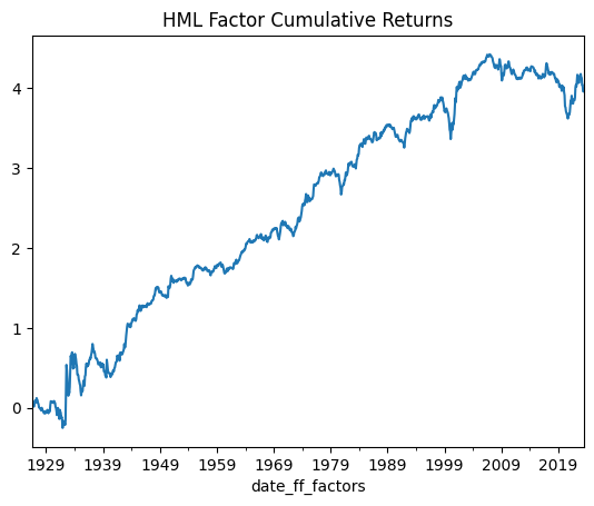
Carhart Four Factor Model
The Carhart Four Factor Model builds on the Fama-French Three Factor model by adding Momentum as an additional explanatory factor. This was formalised in Mark Carhart’s 1997 paper “On Persistence in Mutual Fund Performance”:
The new component “UMD” (Up Minus Down) captures the returns associated with owning companies whose stock prices have risen (winners) versus companies whose prices have fallen (losers). The pioneering paper on Momentum is “Returns to Buying Winners and Selling Losers” by Jegadeesh and Titman (1993).
Momentum
Conceptual basis: Companies that have performed well recently will continue to perform well in the near future.
Potential explanatory theories include behavioural factors such as herding and confirmation bias, investor tendencies towards both underreaction and overreaction, and supply/demand dynamics including indexation effects.
df_c4f_monthly = gff.carhart4Factor(frequency='m')
df_c4f_monthly.set_index('date_ff_factors', inplace=True)
show_me_factor_info('MOM', df_c4f_monthly)
Cumulative Return: 726.44%
Mean Annual Return: 7.53%
Annualised Volatility: 16.31%
Annual Sharpe Ratio: 0.46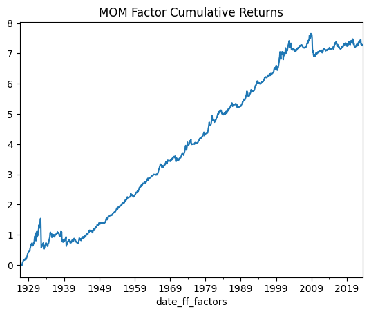
While Momentum has exhibited robust long-term performance, the factor is susceptible to significant crashes. On the logarithmic scale of the chart these crashes appear less severe than they truly were. The max drawdown chart gives a clearer picture:
To compute max drawdown from simple monthly returns, we compound them geometrically and track the running peak.
# MOM column contains simple monthly returns from Ken French's library
mom_gross_returns = (1 + df_c4f_monthly['MOM']).fillna(1)
cumulative_reinvested_return = mom_gross_returns.cumprod()

# Plot the max drawdown time series
((cumulative_reinvested_return - cumulative_reinvested_return.expanding().max()) /
 (cumulative_reinvested_return.expanding().max()) * 100).plot(title='MOM Max Drawdown in %')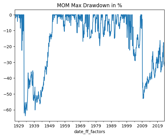
Drawdowns of this magnitude are often cited as problematic for institutional mandates — the exact threshold varies by fund structure, investor base, and stated risk profile, but large peak-to-trough losses typically invite difficult conversations with allocators. The period from 1950 to 2008 looks manageable by this standard. The drawdowns before and after that window are notably deep — a rapid 50% loss over a few months is particularly unpleasant. This underscores one of the principal risks in Momentum investing: the potential for severe crashes, and the time required to recover from them.
Fama-French Five Factor Model
In 2015, Fama and French published an extension adding two new factors:
- Robust Minus Weak (RMW): returns on companies with strong operating profitability minus companies with weak profitability — the “profitability” factor
- Conservative Minus Aggressive (CMA): returns on companies with conservative investment levels minus companies investing aggressively — the “investment” or “capex” factor
Although the addition of these two factors filled gaps in the literature, some academics and practitioners had mixed views. Robeco, one of the larger factor-focused asset managers, noted surprise that Momentum was not formally included as a factor, especially given its explanatory power. Others noted that the Low Volatility factor — which directly contradicts the Market Risk Premium — was not addressed. Nevertheless, the inclusion of Profitability and Investment represented a meaningful enhancement over the Three Factor model.
Profitability (RMW)
Conceptual basis: Companies with higher profit margins earn higher returns than those with lower margins.
Potential explanatory theories: profitable firms tend to be growth firms likely to appreciate; profitable companies may be less volatile and thus not popular for speculation; and profitable firms are less prone to distress.
df_ff5f_monthly = gff.famaFrench5Factor(frequency='m')
df_ff5f_monthly.set_index('date_ff_factors', inplace=True)
show_me_factor_info('RMW', df_ff5f_monthly)
Cumulative Return: 204.1%
Mean Annual Return: 3.4%
Annualised Volatility: 7.69%
Annual Sharpe Ratio: 0.44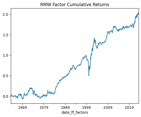
Investment (CMA)
Conceptual basis: Companies reinvesting aggressively tend to underperform those with conservative capital allocation.
Potential explanatory theories: conservative reinvestment may signal disciplined capital allocation, while aggressive capex can signal empire-building or overoptimistic growth forecasts.
show_me_factor_info('CMA', df_ff5f_monthly)Cumulative Return: 200.32%
Mean Annual Return: 3.34%
Annualised Volatility: 7.21%
Annual Sharpe Ratio: 0.46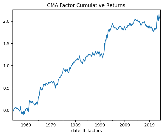
Something interesting: both the Profitability and Investment factors perform well during times of market stress. Here they are plotted alongside the Market return, zoomed into 1999–2022:
title = 'CMA/RMW Returns vs. Market Returns 1999 to 2022'
df_ff5f_monthly[['CMA', 'RMW', 'Mkt-RF']].loc['1999':'2022'].cumsum().plot(title=title)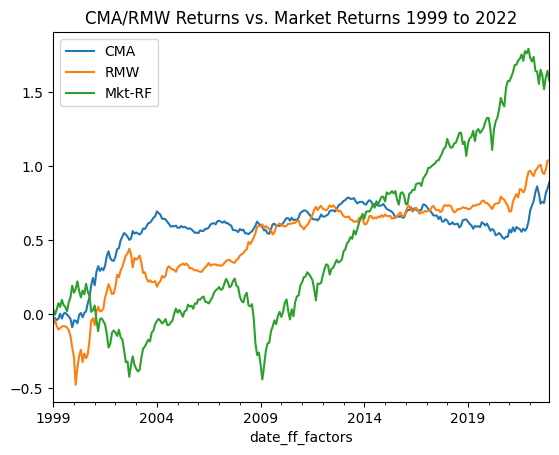
During the dot-com bubble and its aftermath (2000–2003), the market performed poorly while RMW and CMA did quite well. Similar patterns emerge in 2007–2009 and 2022. The correlations of monthly returns for this period confirm it:
df_ff5f_monthly[['CMA', 'RMW', 'Mkt-RF']].loc['1999':'2022'].corr()| CMA | RMW | Mkt-RF | |
|---|---|---|---|
| CMA | 1 | 0.253 | -0.265 |
| RMW | 0.253 | 1 | -0.349 |
| Mkt-RF | -0.265 | -0.349 | 1 |
Some behavioural explanations:
- 2000–2003: Internet stocks with weak (or no) earnings and aggressive capex are sold off. RMW and CMA capture returns for companies with strong earnings and conservative expenditure.
- 2007–2009: The credit crunch causes a flight to quality — investors reallocate to safer companies.
- 2022: Rising interest rates create funding challenges for high-growth companies, echoing the 2000–2003 dynamic.
What’s Next?
In the next post, we’ll look at how to perform factor regressions — measuring a stock’s or portfolio’s exposure to these factors, and why that matters both for alpha-seeking managers and for ETF providers.
The code for this post is available on request.
Footnotes
-
Technically four if you include the risk-free rate. It’s certainly time-varying, but it’s not generally included as a risk factor because its coefficient doesn’t vary in the cross-section of returns — unlike market, size, and value, whose loadings differ across stocks. The risk-free rate’s coefficient is always 1. ↩
-
In general the risk-free return is either the Effective Federal Funds Rate or a similar short-duration deposit facility. I’ve seen people use the US 10-Year Treasury yield as a “risk-free” rate, but that carries meaningful duration risk. A risk-free rate could reasonably be defined differently for each investor based on their investment universe, holding period, and jurisdiction. ↩